SystemVerilog
This is not a complete guide!
This is just here to give some glimpses at some SystemVerilog
additional features.
This is included here more for interest: you
don't need to learn this material but you are welcome to use what
you can if you wish.
You can find the full IEEE standard for SystemVerilog
(legitimately!) via the University's subscription to IEEE Xplore
For design-and-build
SystemVerilog
expands Verilog in numerous ways. A very useful addition is the
declaration (data type)
logic,
which is almost the same as
reg
(which, remember, is not always driven by a physical register)
but can be driven with
assign
too. This is one of the extensions you're most likely to encounter
first if you do this sort of thing in future.
Another new type is
bit
(it can still come in arrays to form variables); these bits always
have binary values and can't adopt
x or
z states.
| type |
Language |
Effect |
States |
| wire aaa; | Verilog | Declare a net: a combinatorial logic value. |
{0, 1, X, Z} |
| reg bbb; | Verilog | A signal which may (or may not) be state holding. | {0, 1, X, Z} |
| logic
… | SystemVerilog | Declare either a net
or a variable, depending on
usage. | {0, 1, X, Z} |
| bit
… | SystemVerilog | Like logic but can
only adopt one of two states. Can still be a multibit variable. | {0, 1} |
- A net is a signal which is not state-holding but can
always be derived from its inputs at any instant.
- A variable is state-holding: typically it is the
output of a D-type flip-flop/register.
These can be assigned by ‘Procedural
Blocks’ to help avoid pitfalls resulting from
potential ambiguities in its predecessor. For example
always_comb
can help to avoid accidental omissions in a sensitivity list, thus:
always_comb
a = b & c;
can replace
always @ (*) a = b & c;
(although there are some subtle
differences here, such as the former also executing at
t = 0).
always_comb
blocks are also sensitive to changes in inputs to any functions called
from within, while
always @ (*)
blocks are not.
This is restricted to combinatorial blocks. Presumably the
idea is to ensure only ‘proper’ code is enclosed, so
providing an additional security check. With
always_comb
the sensitivity list is inferred by the tools (plus a
‘bonus’ execution after
initialisation).
Plus, any particular assigned (written) value can only be assigned
within one such block.
(The Verilog language allows a variable to be written to in multiple
always
blocks: this is generally Bad Practice and will be rejected by
most/all(?) logic synthesizers.)
Danger: a ‘trap’ in Verilog
There is a nasty ‘trap’ in ‘old-fashioned’
Verilog style which, presumably, arises from it beginning as a
Hardware Description Language: this is the inadvertent
introduction of latches.
always @ (*)
if (X) a = b + c;
else if (Y) a = b - c;
Verilog acts as a programming language, where
a will not
change if neither
X nor
Y is
‘true’. This is ‘natural’ in programming but
assumes variable storage: when synthesized this means including
an extra latch structure, which is (almost certainly) unwanted,
and (definitely) expensive in area, power, timing and may introduce
timing (glitch) problems in implementation.
Logic synthesizers typically spot this issue and produce
‘Warning’ messages —
which developers typically ignore!
To avoid problems always include a definition for every output
state in a combinatorial logic description: if/when you don't
care, make this explicit and the synthesizer will (hopefully!) choose
the cheapest possible implementation. Thus:
always @ (*)
if (X) a = b + c;
else if (Y)
a = b - c;
else
a = 'hx;
// Don't care
It's strongly suggested this is applied as a
default:
in all
case
statements too, as a good habit.
Similarly there are also
always_ff and
always_latch
for registers and latches respectively, although these are (arguably)
less of a boon.
Finally (here) there is
final
which is the scheduler's complement to
initial.
This(/these) run(s) after a simulation has ‘$finished’. They can be useful for
(e.g.) outputting results and statistics or closing files. This is
only useful for test code, of course.
initial
in ASICs vs. FPGAs
initial
is used in verification code to run a thread at start-up time. When a
design is synthesised into an FPGA the synthesiser can interpret some
initial
statements and set up the contents of memories and the state of
registers and flip-flops. This is because these values are downloaded
when the FPGA is configured.
In an ASIC there is no downloading! Registers will not be
initialised and (in Verilog terms) start with a value
‘X’.
This can be very important when implementing state machines, et al.
where an active ‘reset’ is usually needed. RAM must also
be actively loaded; ROM contents must have been preprogrammed when the
appropriate macrocell was specified.
There are explicit enumerated types which save listing
definitions by hand.
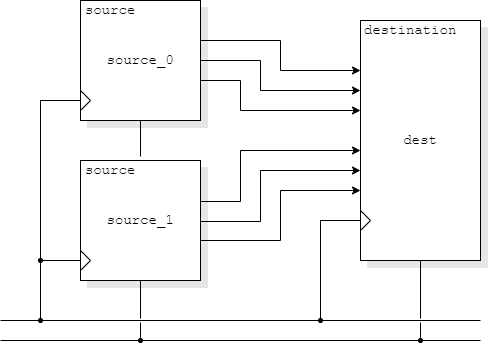
Interfaces
For large hierarchies the inter-block wiring can become very complex
with bundles of buses all heading in the same direction. In old-style
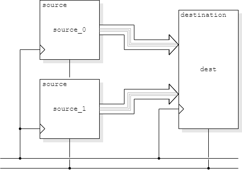
Verilog this gets complicated/messy/error-prone. Interfaces
provide a means of ‘wrapping’ associated signals into more
complex buses which can be connected as single units.
module top();
logic clk;
logic reset;
logic bits_0;
logic bobs_0;
logic pieces_0;
logic bits_1;
logic bobs_1;
logic pieces_1;
source source_0(.clk(clk),
.reset(reset),
.bits(bits_0)),
.bobs(bobs_0)),
.pieces(pieces_0));
source source_1(.clk(clk),
.reset(reset),
.bits(bits_1)),
.bobs(bobs_1)),
.pieces(pieces_1));
destination dest(.clk(clk),
.reset(reset),
.bits_0(bits_0),
.bobs_0(bobs_0),
.pieces_0(pieces_0),
.bits_1(bits_1),
.bobs_1(bobs_1),
.pieces_1(pieces_1));
endmodule : top
module source(input logic clk,
input logic reset,
output logic bits,
output logic bobs,
output logic pieces);
...
endmodule : source
module destination(input logic clk,
input logic reset,
input logic bits_0,
input logic bobs_0,
input logic pieces_0,
input logic bits_1,
input logic bobs_1,
input logic pieces_1);
...
endmodule : destination
interface bundle;
logic bits;
logic bobs;
logic pieces;
endinterface
module top();
logic clk;
logic reset;
bundle stuff_0;
bundle stuff_1;
source source_0(.clk(clk),
.reset(reset),
.stuff_out(stuff_0));
source source_1(.clk(clk),
.reset(reset),
.stuff_out(stuff_1));
destination dest(.clk(clk),
.reset(reset),
.stuff_in_0(stuff_0),
.stuff_in_0(stuff_1));
endmodule : top
module source(input logic clk,
input logic reset,
bundle stuff_out);
...
endmodule : source
module destination(input logic clk,
input logic reset,
bundle stuff_in_0,
bundle stuff_in_1);
...
endmodule : destination
Access to the fields within an interface follows the convention you
might guess at. Thus, for example, in the instance
dest above,
fields can be broken out as
‘stuff_in_0.bits’,
‘stuff_in_0.bobs’
etc.
Structures
Interfaces bundle together associated wiring so multiple buses
can be handled as one entity. Structures serve a similar role
for other elements, such as associated registers. The syntax is very
C-like and should be more or less intuitive for anyone used to
programming.
struct { bit [7:0] opcode; bit [23:0] addr; } IR;
(Nicked definitions from standard.)
typedef struct {
bit [7:0] opcode;
bit [23:0] addr;
} instruction;
// Type defined
instruction IR;
// Stucture variable defined
Arrays
Verilog syntax can be both somewhat confusing and somewhat restrictive
in this area. SystemVerilog at least alleviates some of the
restrictions! First, some terminology:
- An array can be packed
logic [31:0] data;
- or unpacked
logic memory [0:1023];
In both cases the index is expanded across the specified range. The
index can be ascending or descending although it is typically
conventional to number bits-in-a-bus, at least, in a descending
(little-endian) sequence.
A one dimensional packed array (as
here) is sometimes called a ‘vector’. Only certain
data types may be ‘packed’ although these are the elements
you might expect, such as
reg,
logic etc.
The two types can be combined, such as:
logic [31:0] mem [0:1023];
which declares a 1 KiW memory of 32-bit words. Access is then
available with statements such as:
data = mem[addr];
… and this is sometimes referred to explicitly as a
‘memory’.
SystemVerilog allows more detailed indexing so that (for example) a
byte could be extracted from the memory:
data = mem[addr][15:8];
(Note the position of the indices!)
It is possible to have – and combine – multiple packed and
unpacked dimensions in arrays. This can get quite confusing, so
don't be too tempted and take care (and read the documentation!)
before getting in too deeply.
Nesting
SystemVerilog allows modules to be declared within other
modules, limiting their scope accordingly.
Did you know …
Verilog can ‘get at’ any signal using the
appropriate hierarchical name
(with
‘.’
separators).
local_signal = module_X.submodule_Y.signal_of_interest;
This can be handy in verification to ‘probe’ the insides
of nested modules – perhaps with some logic functions.
For verification
The improvement is testbench facilities is probably the most
significant addition. These include (presumably) familiar concepts
such as object-oriented programming and string handling.
Debugging is eased with
assertions (also present
in some earlier Verilog extensions, but not as formalised).
Debug suggestion
Typically bus signals ‘hang around’ even when not in use:
for example a memory address will possibly remain on the address bus
after a transfer is complete. For display and
verification (only) it can be convenient to highlight
the value only during the actual transfer.
A means of doing this is to create (within the testbench) some extra
signals for display purposes. Something like:
assign disp_address = (read || write) ? address : 'hXXXX;
This makes the signal ‘undefined’ (you could choose
Z
if preferred) when not in use which makes the transfers much more
obvious in a trace.

Miscellaneous
Lots of syntactic features (such as
‘x++’)
now work the way you might expect; loops can
break or
continue
and so on. There's plenty more detailed stuff if interested and not
enough time/space here to delve into it all.
Up to Verilog index
Onward to assertions.