Simulation time

As far as physics currently understands time is a single continuous dimension.

Simulation time is discrete but multidimensional! (Short aside: Event Driven Simulation.)

There is a simulation time which represents real delays
- This is available as $time
- Resolution is controllable; may be a fraction of ‘#1’
There is a list of things which happen simultaneously (in a given simulation) timestep
- Some of these are ordered
- e.g. blocking assignments within the same block
- Some are unpredictable
- e.g. blocking assignments different blocks
- There are different phases
- first: all blocking assignments
- second: non-blocking assignments

Naturally, none of this relates to the actual time taken to run the simulation, which depends on how much switching activity takes place in the design.

Assignment timing

Assuming they are scheduled to happen at the same time:

Blocking assignments occur in some order
- the order is only defined within a single statement
Non-blocking assignments happen simultaneously
- first all the results are calculated from the RHS expressions
- then all the LHS variables are altered
Non blocking assignments happen after blocking assignments

Example

always @ (posedge clk) a = b;       // Blocking
always @ (posedge clk) b = a;       // Blocking
always @ (posedge clk) x <= y;      // Non-blocking
always @ (posedge clk) y <= x;      // Non-blocking

After a clock edge:

x and y will have been swapped

but which value depends on the implementation
i.e. which of the blocking statements is scheduled first

However:

always @ (posedge clk)
begin
a = b;
b = a;
end

is entirely predictable – if rather pointless.

Potential pitfall

always @ (posedge clk) x <= a; // Non-blocking
always @ (posedge clk) a = b; // Blocking

In simulation x will always take the value from b.

However a synthesizer will probably see this as two sequential flip-flops.

A synthesized circuit will behave differently from the simulation!

Okay, that's the wrong thing to happen but complaining won't change it.

Guidelines

Use blocking assignments for combinatorial logic
- this should evaluate every time its inputs change
Use non-blocking assignments for D-type (edge-triggered) registers
- typically ‘posedge clk’
Don't mix blocking (=) and non-blocking (<=) assignments ...
- ... to a particular variable
- ... within the same always block
Keep all assignments to a particular variable in the same block
Try to avoid transparent latches^†
always @ (D, En) if (En) Q = D;
- only do this if you must
- easily created accidentally: remember ‘else’s and ‘default’s
- may be functionally harmless but introduce redundant logic
- some tools may produce warnings if you do

^† [Forward reference]

Stylistic pitfall (?)

When simulating synchronous circuit models the most convenient thing to write is:

always @ (posedge clk)
if (count < 9) count <= count + 1; else count <= 0;

‘count’ then changes:

as a result of the clock edge
after the clock edge
at the same time as the clock edge

The resulting trace may be slightly misleading although it is safe.

But what if the inputs (RHS) are generated with a blocking assignment ...

as combinatorial logic? Okay – inputs settled in time
@ (posedge clk) ? Bad news – inputs change before non-blocking statement
(In simulation, maybe not in synthesized logic.)

Therefore keep all blocks and modules in the same style!

This might aid readability …

(Perhaps) the obvious way to stimulate a design may be something like this:

initial clk = 1;
always #5 clk <= !clk;

initial
  begin
  data = 0;
  #10;
  data = 1;
  #10;
  data = 2;
  #10;
  end

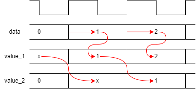
always @ (posedge clk) value_1 <= data;
always @ (posedge clk) value_2 <= value_1;

Unfortunately – because the blocking assignment (data) completes before the non-blocking assignments – this will lead to the following timing relationship:

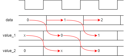
Offsetting input changes slightly from the clock may help.

parameter period = 10; // Makes changes easier

initial clk = 1;
always #(period/2) clk <= !clk;

initial
  begin
  #1; // Inputs delayed
  data = 0;
  #period;
  data = 1;
  #period;
  data = 2;
  #period;
  end

always @ (posedge clk) value_1 <= data;
always @ (posedge clk) value_2 <= value_1;

There are a couple of disadvantages of the form above.

It's easy to compound execution delays accidentally.
The ‘right hand side’of the assignment is evaluated after the clock edge.
- This doesn't matter for constants …
- … but can cause problems with variables which may already have changed.

parameter period = 10; // Makes changes easier

initial clk = 1;
always #(period/2) clk <= !clk;

initial
  begin
  data <= #1 0; // Inertial delay
  #period;
  data <= #1 1;
  #period;
  data <= #1 2;
  #period;
  end

always @ (posedge clk) value_1 <= #1 data;
always @ (posedge clk) value_2 <= #1 value_1;

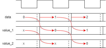
The evaluation here takes place at the clock edge: it is just the result assignment which is delayed.
Suggest that this is clearer!

The ‘pipeline’ behaves as one might expect.
The input traces are easier to spot.

Rather than inserting explicit delay times it may be more robust to count the clock edges. The ‘@’ symbol means ‘at the next event from the following list’ so: ‘@ (posedge clk)’ means ‘wait until the next active clock edge’ — this will always keep execution in synchronisation with the clock.

‘repeat (10) @ (posedge clk)’ will, of course wait for the tenth successive clock edge etc.

Delays

Delays use a syntax ‘#<value>’
Delays can be added to a model in various ways.
- They will not be synthesized and cannot be relied upon for functionality.

Here are some convenient methods:

#20 a = l; // Delay in execution of sequential block

wire #4 q; // Declare a ‘net delay’ ...
assign q = a & b; // q changes 4 timesteps after an input change

register <= #10 input_value; // Propagation delay on signal

Uses include

Sequencing I/O in a test run
Modelling ‘real’ components
- e.g. external memory read delay in lab. system (> clock period)
‘Cosmetic’ delays to make waveform traces more readable

Delays

Time is modelled in two ways:

advancing to the next timestep
iterating over things which happen at the same time

Examples:

initial
begin
a = 0;
#10;
a = 1;
end

assign b = !a; assign c = !b;

Time	action
0	a = 0
0	b = 1
0	c = 0
10	a = 1
10	b = 0
10	c = 1

At any point there is only one thing which is scheduled to happen, but a change schedules a(n immediate) change on b, etc.

initial
begin
a = 0;
#10;
a = 1;
end

assign #5 b = !a;
assign #6 c = !b;

Time	action
0	a = 0
5	b = 1
10	a = 1
11	c = 0
15	b = 0
21	c = 1

Delays can alter when switching occurs.

Delays can also be inserted within assignments to delay the assignment without retarding the flow of execution, e.g.:

a <= #10 b;

Same unit: different delays

For added veracity it is possible to specify different rising, falling and turn-off delays for a signal by listing these in brackets. E.g.

#(3,2)

means a rising delay of 3, a falling delay of 2. The turn-off delay has not been specified so defaults to the minimum of these (if appropriate).

Glitches

‘Glitches’ are brief signal changes which result from signal races through combinatorial logic; they will only be visible in simulation if gates (or other logic blocks) include delay models. Thus they will not (typically) appear in an abstracted simulation.

Glitches may appear in more detailed models, including a netlist extracted from a synthesized design: i.e. one which includes details of the actual circuits and delays. This could cause problems running the same simulation successfully as previously, depending on how the testbench is constructed. There is a little bonus page about this here.

Up to simulation

Back to parallelism in simulation

Forward simulation events

Bonus pages

Event Driven Simulation

Trouble with glitches